XPCS Analysis 8-ID
This Wiki page is dedicated towards providing documentation on 8-ID XPCS Data Analysis, Visualization and some inner details of what is involved in the analysis. While mostly the documentation is given below, there are also some PDF documents with details.
Overview
The sections below provide description of Visualization of XPCS results followed by details on Data Reduction/Analysis of Raw Data to yield Correlation functions.
XPCS metadata and results are primarily saved into a HDF5 file format based on a Data Exchange format defined at the APS.
MetaData File (HDF5)
The concept is as follows: There are groups in the HDF5 file that are part of the Data Acquisition and these are categorized into the following:
/measurement
/measurement/instrument
/measurement/instrument/acquisition/
/measurement/instrument/detector/
/measurement/instrument/detector/roi/
/measurement/instrument/detector/kinetics/
/measurement/instrument/source_begin/
/measurement/sample/
The above groups each contain several HDF5 datasets or parameters which have a scalar, vector, ND arrays or string attributes. The above are present in every metadata HDF5 file associated with each data acquisition. This file is saved in the same directory/folder as the raw detector images file itself.
Analysis Parameters (XPCS Group)
When a data set is processed which primarily means some sort of a correlation analysis, then the parameters that are needed to analyze the data such as:
- user defined mask
- wave vector maps (called as qmaps) where each wave vector or an azimuthal angle is characterized by a unique integer in what is called as a digitized map
- look up table that links the integers in the qmaps to the q/phi values
- Start and end frame numbers to be processed which could be a subset of the frames collected
- More intricate (meaning ones that are not changed from their defaults often) analysis parameters such as the multitau delay level, striding and averaging frames prior to correlation
- location of the file in the local as well as in a remote file system
- A very critical field which defines where the output of the computation - the results - are saved in the HDF5 file.
The above parameters (data sets) are saved in the HDF5 file in a special group called "/xpcs". Often, a user analyzes a given data set more than once if not several times which could each be under different conditions such as varying one or more of the above analysis parameters. While there might be a short sighted convenience seen in keeping these different analysis into separate HDF5 files, the concept of maintaining groups in the same HDF5 file has a higher value as the user will readily know all the different analysis or processing that are done to a given data set.
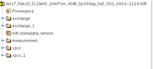
Embracing that idea, the current implementation defines the first time analysis group as "/xpcs" and the output of this analysis is saved into a group that is defined under "/xpcs/output_data" which usually points to a group named "/exchange".
For every subsequent analysis that is performed, the XPCS group is called "/xpcs_N" where N=1,2,3,4,..... In the same way as described above, "/xpcs_N/output_data" points to "/exchange_N".
Result Structure (HDF5 EXCHANGE Group)
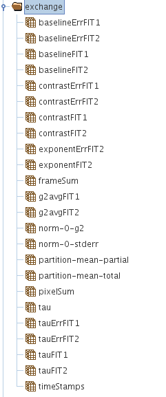
The group called /exchange or /exchange_N in general, has all the analysis results and the fitting results of the correlation analysis in cases when fitting has been performed.
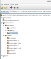
A picture showing what is in the /exchange group is shown.
A picture showing the case when multiple /xpcs and /exchange exist as a result of multiple analyses that has been down is shown.
- There are functions that are available to place the entire data structure into the Matlab workspace for processing that the user might want to do. The function is called as follows (as a default) with the HDF5 file as the only argument in which case it will open the default "/xpcs" group. Recently, a new function has been added called "select_xpcs_group" in which the user could specify a second argument called "first" or "last" which will then select the first which is "/xpcs" or the last which is "/xpcs_N" where N is the highest number found in that HDF5 file.
- viewresultinfo.result = loadhdf5result('FeO_20nm_film5_44p90mm_027_0001-0212.hdf');
- Alternatively, the user could call the above function in the following way in which case it would open "/xpcs_3" in the example below.
viewresultinfo.result = loadhdf5result('FeO_20nm_film5_44p90mm_027_0001-0212.hdf','/xpcs_3');
- A function called hdf5_find_group_suffix('FeO_20nm_film5_44p90mm_027_0001-0212.hdf','/xpcs') would return an integer N where N is the total number of "/xpcs" groups that are present in the HDF5 file.
Result Structure (.mat File)
While the above described HDF5 format offers several advantages and convenience, some times it is convenient to save the results into a native .mat file, which is the binary format of Matlab. (Note that as of R2016 or so, .mat is also internally a HDF5 file but the groups and data sets in such a file are not seen outside). The .mat file can be read using native Matlab funcion "load".
- load SPS64_140k_200nm_154C_F2_TimeSeries_avg.mat
OR
- load('SPS64_140k_200nm_154C_F2_TimeSeries_avg.mat')
will load the parameters saved in the .mat file into the workspace.
- Another useful command when using a .mat file is matfile which shows what is inside the file without loading any of it to the workspace.
matfile('SPS64_140k_200nm_154C_F2_TimeSeries_avg.mat')
Summary of Result Structure
Irrespective of the results being saved in HDF5 or .mat format, the respective functions (loadhdf5result and load) described above offers the exact same result structure in the work space so that the rest of the code (plotting, fitting, visualization) are agnostic to the format. The standard name for the structure in the workspace, when the functions are called as described above (especially for the HDF5, note viewresultinfo.result). This is a structure in Matlab which is a way to store several parameters comprising of numerics and strings in a hierarchical manner.
VIEW_XPCSGUI_RESULTS Visualization Package
- A visualization software package is provided that is called "VIEW_XPCSGUI_RESULTS" which is maintained in the APS Internal Version Control repository Subversion. The package is meant to handle results from either HDF5 file or a .mat file.
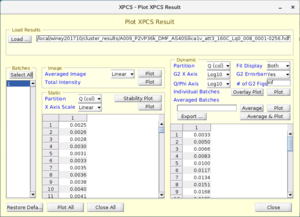
- The package primarily comprises of a GUI called "viewresult" which has easy pre-defined plots for visualizing typical parameters such as the SAXS I(q), Average intensity variation with time, I(q,t) which shows the SAXS variation with time and most importantly the time correlation functions, g2, as a function of q and phi.
How to process the Result Structure?
Below, a typical result structure is shown under two different scenarios.The variables are given names that are some what self-explanatory but not obviously always. The general format for the different parameters involving q/phi are (#q x #phi x #dt). In cases where there is only one phi partition, it will look like (#q x 1 x #dt). These two cases are shown below along with a description to the right of what the parameter means to a user.
Files NOT containing azimuthal (phi) bins
viewresultinfo.result
ans =
           hdf5_filename: {'XR6_25p0C_Sq1_001_0001-0074.hdf'}
   result_group_location: {'/exchange'}
         xpcs_group_name: {'/xpcs'}
                staticQs: {[90x1 double]} %%list of q-values in the static partition
               dynamicQs: {[18x1 double]} %%list of q-values in the dynamic partition
              staticPHIs: {[90x1 double]} %%list of PHI-values in the static partition
             dynamicPHIs: {[18x1 double]} %%list of PHI-values in the dynamic partition
                     aIt: {[1300x1340 double]} %%2-d image of average intensity over all frames
          totalIntensity: {[64x1 double]} %%total intensity, one data point per frame (per kinetics slice for kinetics mode)
              timeStamps: {[64x1 double]} %%time stamp for each frame
            framespacing: {[1.289641633866325e+00]} %% constant spacing in time (sec) between frames
      StdDevframespacing: {[1.222323102678448e-02]} %%standard deviation in the time spacing (in sec)
                   delay: {[19x1 double]} %%time delay (sec) for the g2 plots
            darkAverages: {[NaN]} %%does not exist
              darkStdDev: {[NaN]} %%does not exist
                   Iqphi: {[90x1 double]} %%I(q) - time averaged
                  Iqphit: {[90x1x10 double]} %%I(q) with time - stability plot
                   g2avg: {[18x1x19 double]} %% measured g2 vs delay time (num of dyn qs x num dyn phis x number of delay)
matlab syntax: squeeze(viewresultinfo.result.g2avg{1}(1,1,:)) %to read #q=1,#phi=1, all the dt's (same for g2avgErr)
               g2avgErr: {[18x1x19 double]} %%g2 error bars
                   %%%FIT1 is simple exp
               g2avgFIT1: {[18x1x19 double]} %%simple exp fitted values of g2
                 tauFIT1: {[18x1 double]} %%tau values at each dynamic q for simple exp
              tauErrFIT1: {[18x1 double]}%%tau error values at each dynamic q for simple exp
            baselineFIT1: {[18x1 double]} %%baseline values at each dynamic q for simple exp
         baselineErrFIT1: {[18x1 double]} %%baseline error values at each dynamic q for simple exp
            contrastFIT1: {[18x1 double]} %%contrast values at each dynamic q for simple exp
         contrastErrFIT1: {[18x1 double]} %%contrast error values at each dynamic q for simple exp
                %%%FIT2 is stretched exp
               g2avgFIT2: {[18x1x19 double]} %%stretched exp fitted values of g2
                 tauFIT2: {[18x1 double]} %%tau values at each dynamic q for stretched exp
              tauErrFIT2: {[18x1 double]} %%tau error values at each dynamic q for stretched exp
            baselineFIT2: {[18x1 double]} %%baseline values at each dynamic q for stretched exp
         baselineErrFIT2: {[18x1 double]} %%baseline error values at each dynamic q for stretched exp
            contrastFIT2: {[18x1 double]} %%contrast values at each dynamic q for stretched exp
         contrastErrFIT2: {[18x1 double]} %%contrast error values at each dynamic q for stretched exp
            exponentFIT2: {[18x1 double]} %%exponent values at each dynamic q for stretched exp
         exponentErrFIT2: {[18x1 double]} %%exponent error values at each dynamic q for stretched exp
%%%%%%%%%%%%%%%%%%%%%%%%%%%%%%%%%%%%%%%%%%%%%%%%%%%%%%%%%%%%%%%%
Files containing azimuthal (phi) bins
viewresultinfo.result
ans =
           hdf5_filename: {'FeO_20nm_film5_44p90mm_027_0001-0212.hdf'}
   result_group_location: {'/exchange'}
         xpcs_group_name: {'/xpcs'}
                staticQs: {[72x60 double]}
               dynamicQs: {[24x1 double]}
              staticPHIs: {[72x60 double]}
             dynamicPHIs: {[24x1 double]}
                     aIt: {[1300x1340 double]} %%2-d image of average intensity over all frames
          totalIntensity: {[202x1 double]} %%total intensity, one data point per frame (per kinetics slice for kinetics mode)
              timeStamps: {[202x1 double]} %%time stamp for each frame
            framespacing: {[3.132541805357482e+00]} %% constant spacing in time (sec) between frames
      StdDevframespacing: {[1.387878691212486e-02]} %%standard deviation in the time spacing (in sec)
                   delay: {[25x1 double]} %%time delay (sec) for the g2 plots
            darkAverages: {[NaN]} %%does not exist
              darkStdDev: {[NaN]} %%does not exist
                   Iqphi: {[72x60 double]} %%I(q) - time averaged
                  Iqphit: {[72x60x10 double]} %%I(q) with time - stability plot
                   g2avg: {[24x1x25 double]} %% measured g2 vs delay time (num of dyn qs x num dyn phis x number of delay)
% matlab syntax: squeeze(viewresultinfo.result.g2avg{1}(3,11,:)) %to read #q=3,#phi=11, all the dt's (same for g2avgErr)
                g2avgErr: {[24x1x25 double]} %%g2 error bars
                       %%%FIT1 is simple exp
               g2avgFIT1: {[24x1x25 double]} %%simple exp fitted values of g2
                 tauFIT1: {[24x1 double]} %%tau values at each dynamic q for simple exp
              tauErrFIT1: {[24x1 double]} %%tau error values at each dynamic q for simple exp
            baselineFIT1: {[24x1 double]} %%baseline values at each dynamic q for simple exp
         baselineErrFIT1: {[24x1 double]} %%baseline error values at each dynamic q for simple exp
            contrastFIT1: {[24x1 double]} %%contrast values at each dynamic q for simple exp
         contrastErrFIT1: {[24x1 double]} %%contrast error values at each dynamic q for simple exp
                       %%%FIT2 is stretched exp
               g2avgFIT2: {[24x1x25 double]} %%stretched exp fitted values of g2
                 tauFIT2: {[24x1 double]} %%tau values at each dynamic q for stretched exp
              tauErrFIT2: {[24x1 double]} %%tau error values at each dynamic q for stretched exp
            baselineFIT2: {[24x1 double]} %%baseline values at each dynamic q for stretched exp
         baselineErrFIT2: {[24x1 double]} %%baseline error values at each dynamic q for stretched exp
            contrastFIT2: {[24x1 double]} %%contrast values at each dynamic q for stretched exp
         contrastErrFIT2: {[24x1 double]} %%contrast error values at each dynamic q for stretched exp
            exponentFIT2: {[24x1 double]} %%exponent values at each dynamic q for stretched exp
         exponentErrFIT2: {[24x1 double]} %%exponent error values at each dynamic q for stretched exp
Averaging and Averaged Result Structure
Average of several individual batches each with a set of g2 at different q's (done using the GUI, select a set of batches to average and then use the Export tab at the right of the GUI to save the average results to a file. If not exported, the average g2s are plotted but not saved. Such an exported file contains the results of all the files, a field called viewresultinfo.result.batches2average: [1 2 3 4] which shows the batches that were selected by the user to average. The averaged results are always stored as a .mat file and HDF5 format is not made available so far (no reason except no major drive from any user)
A typical structure of such a file is as shown below:
load SPS64_140k_200nm_154C_F2_TimeSeries_avg.mat will return viewresultinfo to the Matlab workspace which looks as shown below.
Skip several lines to see the fields containing "Batchavg"
viewresultinfo =
result: [1x1 struct]
viewresultinfo.result ans =
                hdf5_filename: {1x4 cell}
        result_group_location: {'/exchange'  '/exchange'  '/exchange'  '/exchange'}
              xpcs_group_name: {'/xpcs'  '/xpcs'  '/xpcs'  '/xpcs'}
                     staticQs: {[54x60 double]  [54x60 double]  [54x60 double]  [54x60 double]}
                    dynamicQs: {[18x1 double]  [18x1 double]  [18x1 double]  [18x1 double]}
                   staticPHIs: {[54x60 double]  [54x60 double]  [54x60 double]  [54x60 double]}
                  dynamicPHIs: {[18x1 double]  [18x1 double]  [18x1 double]  [18x1 double]}
                          aIt: {[1300x1340 double]  [1300x1340 double]  [1300x1340 double]  [1300x1340 double]}
               totalIntensity: {[256x1 double]  [256x1 double]  [256x1 double]  [256x1 double]}
                   timeStamps: {[256x1 double]  [256x1 double]  [256x1 double]  [256x1 double]}
                 framespacing: {1x4 cell}
           StdDevframespacing: {1x4 cell}
                        delay: {[27x1 double]  [27x1 double]  [27x1 double]  [27x1 double]}
                 darkAverages: {[NaN]  [NaN]  [NaN]  [NaN]}
                   darkStdDev: {[NaN]  [NaN]  [NaN]  [NaN]}
                        Iqphi: {[54x60 double]  [54x60 double]  [54x60 double]  [54x60 double]}
                       Iqphit: {[54x60x10 double]  [54x60x10 double]  [54x60x10 double]  [54x60x10 double]}
                        g2avg: {[18x1x27 double]  [18x1x27 double]  [18x1x27 double]  [18x1x27 double]}
                     g2avgErr: {[18x1x27 double]  [18x1x27 double]  [18x1x27 double]  [18x1x27 double]}
                    g2avgFIT1: {[18x1x27 double]  [18x1x27 double]  [18x1x27 double]  [18x1x27 double]}
                      tauFIT1: {[18x1 double]  [18x1 double]  [18x1 double]  [18x1 double]}
                   tauErrFIT1: {[18x1 double]  [18x1 double]  [18x1 double]  [18x1 double]}
                 baselineFIT1: {[18x1 double]  [18x1 double]  [18x1 double]  [18x1 double]}
              baselineErrFIT1: {[18x1 double]  [18x1 double]  [18x1 double]  [18x1 double]}
                 contrastFIT1: {[18x1 double]  [18x1 double]  [18x1 double]  [18x1 double]}
              contrastErrFIT1: {[18x1 double]  [18x1 double]  [18x1 double]  [18x1 double]}
                    g2avgFIT2: {[18x1x27 double]  [18x1x27 double]  [18x1x27 double]  [18x1x27 double]}
                      tauFIT2: {[18x1 double]  [18x1 double]  [18x1 double]  [18x1 double]}
                   tauErrFIT2: {[18x1 double]  [18x1 double]  [18x1 double]  [18x1 double]}
                 baselineFIT2: {[18x1 double]  [18x1 double]  [18x1 double]  [18x1 double]}
              baselineErrFIT2: {[18x1 double]  [18x1 double]  [18x1 double]  [18x1 double]}
                 contrastFIT2: {[18x1 double]  [18x1 double]  [18x1 double]  [18x1 double]}
              contrastErrFIT2: {[18x1 double]  [18x1 double]  [18x1 double]  [18x1 double]}
                 exponentFIT2: {[18x1 double]  [18x1 double]  [18x1 double]  [18x1 double]}
              exponentErrFIT2: {[18x1 double]  [18x1 double]  [18x1 double]  [18x1 double]}
              resultfilenames: {1x4 cell}
   Start_Data_Collection_Time: {1x4 cell}
     End_Data_Collection_Time: {1x4 cell}
                batchinfoFile: {'foo'  'foo'  'foo'  'foo'}
                     specfile: {1x4 cell}
               specdata_scanN: {' 28'  ' 30'  ' 32'  ' 34'}
                 datafilename: {1x4 cell}
                   ndata0todo: {[11]  [11]  [11]  [11]}
                 ndataendtodo: {[266]  [266]  [266]  [266]}
                   batches2average: [1 2 3 4]
                   g2Batchavg: [18x1x27 double]
                   g2BatchavgErr: [18x1x27 double]
                   g2BatchavgFIT1: [18x1x27 double]
                   baselineBatchavgFIT1: [18x1 double]
                   contrastBatchavgFIT1: [18x1 double]
                   tauBatchavgFIT1: [18x1 double]
                   baselineErrBatchavgFIT1: [18x1 double]
                   contrastErrBatchavgFIT1: [18x1 double]
                   tauErrBatchavgFIT1: [18x1 double]
                   g2BatchavgFIT2: [18x1x27 double]
                   baselineBatchavgFIT2: [18x1 double]
                   contrastBatchavgFIT2: [18x1 double]
                   tauBatchavgFIT2: [18x1 double]
                   exponentBatchavgFIT2: [18x1 double]
                   baselineErrBatchavgFIT2: [18x1 double]
                   contrastErrBatchavgFIT2: [18x1 double]
                   tauErrBatchavgFIT2: [18x1 double]
                   exponentErrBatchavgFIT2: [18x1 double]
The fields above that contain "Batchavg" in the names are the average of the parameters and the names are obvious with same description as above.
ASCII Conversion of Result Files
The files shown below are part of the VIEW_XPCSGUI_RESULTS package.
The first file below is the file to be used which will call the file listed below. This set of functions will be used to convert single result files (resulting from the analysis of a single data set) that are not averaged.
- input_function_AsciiwithFIT_from_xpcsgui.m
- function_AsciiwithFIT_from_xpcsgui.m
The first file below is the file to be used which will call the file listed below. This set of functions will be used to convert averaged result files (resulting from the average of several individual analysis files).
- input_function_AsciiAvg_from_xpcsgui.m
- function_AsciiAvgwithFIT_from_xpcsgui.m
- function_AsciiAvg_from_xpcsgui.m (this is a less used file which is same as the one above except it does not save the fitting results. This is provided as some users like to fit by themselves.
Ascii_from_xpcsgui.m %-- Converts a single batch result file to 4 files named as
                           %.IQASCII,.g2ASCII,.tauFIT1ASCII,tauFIT2ASCII
                           % IQASCII: 3 columns: q,I(q),error in I(q)
                           %.g2avgASCII: delay as the 1st column, measured
                           %g2@q=1, measured error in g2@q=1. The 2 columns are
                           %repeated for all q's. So for 18 q's, there
                           %should be 1 for delay+18*2=37 columns
                           %.tauFIT1ASCII: q, tau, error in tau
                           %.tauFIT2ASCII: q, tau, error in tau, exponent,
                           %error in exponent
AsciiwithFIT_from_xpcsgui.m %-- Converts a single batch result file to 4 files named as
                           %.IQASCII,.g2ASCII,.tauFIT1ASCII,tauFIT2ASCII
                           % IQASCII: 3 columns: q,I(q),error in I(q)
                           %.g2ASCII: delay as the 1st column, measured
                           %g2@q=1, measured error in g2@q=1, g2FIT1,g2FIT2. The 4 columns are
                           %repeated for all q's. So for 18 q's, there
                           %should be 1 for delay+18*4=73 columns
                           %.tauFIT1ASCII: q, tau, error in tau
                           %.tauFIT2ASCII: q, tau, error in tau, exponent,
                           %error in exponent
AsciiAvg_from_xpcsgui.m %-- Converts the averaged batch result file to 4 files named as
                           %.IQASCII,.g2avgASCII,.tauavgFIT1ASCII,tauavgFIT2ASCII
                           % IQASCII: 3 columns: q,I(q),error in I(q)
                           %.g2avgASCII: delay as the 1st column, averaged
                           %g2@q=1, averaged g2 error in g2@q=1, g2avgFIT1,g2avgFIT2. The 4 columns are
                           %repeated for all q's. So for 18 q's, there
                           %should be 1 for delay+18*4=73 columns
                           %.tauavgFIT1ASCII: q, tau, error in tau
                           %.tauavgFIT2ASCII: q, tau, error in tau, exponent,
                           %error in exponent
%%%%%%%%%%%%%%%%%%%%%%%%%%%%
More Documentation
- A document describing the procedure for using XPCSGUI2 software package can be viewed or downloaded from here [1].
- A document describing a lot of details of XPCS analysis process can be viewed or downloaded from here [2].
Things to follow
The above is hopefully helpful as a documentation. I hope to add more things as and when time permits.


