Difference between revisions of "LaueGo"
m (→Index Tab) |
|||
| (4 intermediate revisions by the same user not shown) | |||
| Line 42: | Line 42: | ||
<br clear = all> | <br clear = all> | ||
== | == Operations == | ||
=== Index Tab === | |||
''Main Article: [[Single Laue Image Analysis with LaueGo]]'' | ''Main Article: [[Single Laue Image Analysis with LaueGo]]'' | ||
===== Displaying and indexing a single image ===== | |||
===== Strain Refinement===== | |||
===== Display Tables ===== | |||
=== Strain Refinement=== | |||
There is a popup "Display Tables..." which will allow you to easily see tables of information concerning fitted peaks, indexed peaks, strain refined peak, ... | |||
=== | === E scans Tab === | ||
The "E scans" tab is used for data that was taken by scanning energy. It's main function is to make Q-distrbutions. | The "E scans" tab is used for data that was taken by scanning energy. It's main function is to make Q-distrbutions. | ||
First you must push the "Set UpNew E-W scan...". | First you must push the "Set UpNew E-W scan...". | ||
: Enter a title for you plots | |||
: Enter a d-spacing (needed to calulate strain, optional) | |||
: make up a folder name, something short and without spaces. | |||
: PUSH the button labeled "Enter Values, then click here" !!! | |||
If you do not know the preferred d-spacing, just leave it as "Inf". | If you do not know the preferred d-spacing, just leave it as "Inf". | ||
| Line 77: | Line 67: | ||
You can now create a Q-distribution by pushing "Make Q-Depth Surface" | You can now create a Q-distribution by pushing "Make Q-Depth Surface" | ||
== | ===== Masking ===== | ||
Sometimes when evaluating a Q-distribution, it is desirable to only process part of an image, e.g. only get the Q-distribution for those pixels near a particular peak. The way to do this is by maskigng. First you need to get a "white" beam image. Since you probably only have an energy scan, just use the "Make a Pseudo White Image" to add up all of the measured energies to make a "white" image. Second push the "Make a Mask" and select the white beam image. Using the marquee you can add or subtract pixels from the mask. You can also use the "New Freehand" button in the top left of the mask image to select pixels using a freehand curve. When you are done setting the pixels, simply close the image plot (push the red dot at top left corner) to finish making the mask. Note that the top of this window says "Close Me When Done". If you wish to change a mask, just push the "Make a Mask" button again and you will be prompted for a mask to edit. | |||
=== Details Tab === | === Details Tab === | ||
Latest revision as of 17:26, 19 August 2013
LaueGo is the main software package for micro-diffraction data analysis and visualization at 34ID-E. It is implemented based on Igor Pro, which runs on both PC and Mac.
LaueGo is developed by Jon Tischler, and distributed freely to all 34ID-E users.
Download and Installation
The package can be downloaded from its Github page (click "Download ZIP" on the right side of the page). Please follow the installation guide to finish your installation.
Basic Setup
The LaueGo Panel
The first step is to load the micro-diffraction procedures. If there is no menu labeled "LaueGo", then you need to do this. Select the menu "Analysis->Packages-> LaueGo", then select your image file format (HDF5 by default); this loads the basic procedures and will put up the LaueGo Panel. If the "LaueGo" menu already is up, then select the menu "LaueGo -> LaueGo Panel". You can always do this to retrieve the LaueGo Panel or to bring it to the front.
Set up geometry
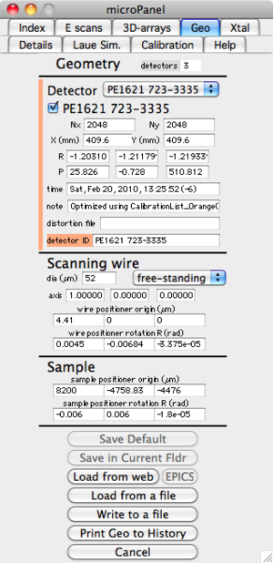
Before almost anything can be done, the calibration parameters also refered to as geometry parameters are needed. These can be set from the "micro" menu, but the easiest way is to use the "Geo" tab on the microPanel. When you select the Geo tab, the current geometry parameters are shown. These geometry parameters describe the location and orientation of all detectors, and also the location and orientation of the scanning wire. Look at the values in the Geometry panel and decide if they are correct. If you want to change them, there are various ways to do that. The simplest way to set the geometry parameters is to load the values from a file. Push the button labeled "Load from a file" and select the appropriate geometry file, it probably starts with "geo" and ends with ".txt" (old format) or ".xml" (new format). You should have been given a geometry file with your data.
An alternative is to use the web server, this uses a date to fetch the geometry values from a web server at APS. Push the button labeled "Load from web". A dialog will then come up asking you to choose an image file. The program gets the date from this image and then asks the web server for the latest geometry parameters that were measured earlier than this date. You can either save the values for use, or reject them by pushing Cancel. If you retrieve the geometry from the web, you shold probably then "Write to a file" too.
It is also possible to load the geometry values from EPICS, but this is probably disabled, and not too useful anyhow.
NOTE: If you change any of the geometry parameters the Save button changes to "Save Default (Needed)" and turns green. So you need to either push the Save button or Cancel (to reject the changes).
The "Save in Current Fldr" button allows you to have these geometry parameters only apply to the data in the current Igor data folder (as shown in the Igor data browser, NOT your data folder on the disk), you will generaly not want this.
The button "Write to a file", writes the current geoemtry values to a text file that can be later read using the "Load from a file" button
The final button on this panel is "Print Geo to History", this prints the current geometry values to the Igor History window. This is not generally needed, but sometimes useful.
Define crystal lattice
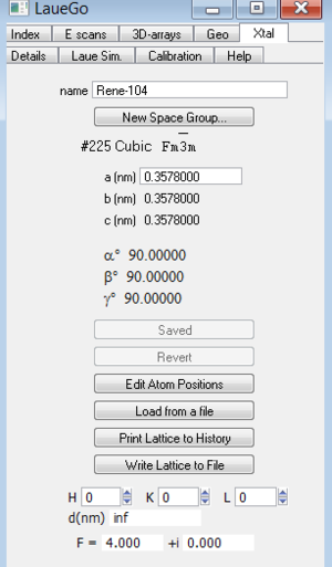
Before you can index a pattern, you must specify the crystal structuere. Do this by choosing the "Xtal" tab in the microPanel. Although the numbers can be entered by hand, it is usually best to enter them by selecting the "Load from a file" button. Remeber to push the "Save (Needed)" button to accept the loaded (or changed) lattice values.
This panel also contains a convienent tool for calculating a d-spacing or atomic structure factor. Just enter the h,k,l values and you will see the d-spacing, and F. The F is calculated assuming that the atomic structure factor is just the atomic number Z.
Operations
Index Tab
Main Article: Single Laue Image Analysis with LaueGo
Displaying and indexing a single image
Strain Refinement
Display Tables
There is a popup "Display Tables..." which will allow you to easily see tables of information concerning fitted peaks, indexed peaks, strain refined peak, ...
E scans Tab
The "E scans" tab is used for data that was taken by scanning energy. It's main function is to make Q-distrbutions.
First you must push the "Set UpNew E-W scan...".
- Enter a title for you plots
- Enter a d-spacing (needed to calulate strain, optional)
- make up a folder name, something short and without spaces.
- PUSH the button labeled "Enter Values, then click here" !!!
If you do not know the preferred d-spacing, just leave it as "Inf".
You can now create a Q-distribution by pushing "Make Q-Depth Surface"
Masking
Sometimes when evaluating a Q-distribution, it is desirable to only process part of an image, e.g. only get the Q-distribution for those pixels near a particular peak. The way to do this is by maskigng. First you need to get a "white" beam image. Since you probably only have an energy scan, just use the "Make a Pseudo White Image" to add up all of the measured energies to make a "white" image. Second push the "Make a Mask" and select the white beam image. Using the marquee you can add or subtract pixels from the mask. You can also use the "New Freehand" button in the top left of the mask image to select pixels using a freehand curve. When you are done setting the pixels, simply close the image plot (push the red dot at top left corner) to finish making the mask. Note that the top of this window says "Close Me When Done". If you wish to change a mask, just push the "Make a Mask" button again and you will be prompted for a mask to edit.
Details Tab
- Review depth-reconstruction summaries. The "Load Recon Summary" loads the summary file from a depth reconstruction. With the reconstructed images from each wire scan you will find a text file with a name like "WW_1_summary.txt". This file sumarizes the result of a wire scan. The button "Load Recon Summary" will select a summary file, load it, and display the total intensity vs. depth for that wire scan. If you need to re-plot the intensity vs. depth for a loaded summary use the following button "Re-Plot Summary".
- Make a movie out of a series of images.
- Sum over multiple images.
- Extract single images from fly-scan data files.
Laue Sim. Tab
Makes a simulated Laue pattern. If you have already indexed the pattern the Laue pattern should be oriented with the simulated indexed pattern.
3D-Arrays Tab
Calibration Tab
Functions used for calibrating beamline geometries, used by beamline staff.

